


Excel
A fixed-rate mortgage is a loan where the installments are equal during the whole repayment period. You may choose this loan to have more predictability within your finances by paying the same amount each time.
Below you’ll see how to put up an overview of a fixed-rate mortgage in a spreadsheet.
Excel Instruction
Making an Overview of a Fixed-rate Mortgage
- 1.
- Open a new spreadsheet and enter the values for the “loan amount”, “interest”, “repayment period” and “installments”.
- 2.
- Set up the template for the table. You’ll need columns representing “years”, “remaining loan”. “amount of interest”, “principal payments” and “installment”. The number of rows is determined by the length of the repayment period.
- 3.
- Enter the formulas in year 1, as well as the remaining loan in year 2.
- 4.
- Copy the formulas of the corresponding columns all the way down to the last payment row.
- 5.
- Sum the columns “amount of interest”, “principle payment” and “installments”.
Example 1
You are taking up a $ fixed-rate mortgage, with an interest of over a twenty-year period. Make a table with an overview of the loan in Excel.
With this loan the installments will be $. You can read more about how to calculate the installments here.
- 1.
- The first thing you do is to enter the relevant numbers for your loan:
- 2.
- Then you make the template. You need the following columns “years”, “remaining loan”, “amount of interest”, “principal payments” and “installment”.
Because the repayment period is 20 years, you’ll need 20 rows in the table:
- 3.
- The remaining loan the first year is the original loan amount, and has already been written in cell
B1. Therefore, write the following in cellB6:=B3
The amount of interest will correspond to the remaining loan that year multiplied by the interest. Write the following in cell
C6:=B6*$B$2
Note! Remember to use a $-sign in
Excelwhen you don’t want the cell reference to change when copying formulas.The principal payment will stay the same the whole repayment period. The amount can be found in cell
E1. Write the following in cellE6:=$E$1
The only cell left in the first row is the installment amount. You know that the principal payment is the sum of the interest amount and the installment. Therefore the installment equals to the principal payment subtracted by the interest. Write the following formula in the cell:
=E6-C6
Before you start copying formulas you need to make a formula for the remaining loan in the second year. Remember that only the installment goes to repay the loan. So the remaining loan in year 2 will equal to the remaining loan in year 1 subtracted by the installment of year 1. Below you’ll find a collection of the formulas:
- 4.
- Now you can take advantage of
Excel’s clever functionality by marking cells containing formulas, and then pull it downwards in the column. Make sure that you only mark cellB7in the remaining loan column. The reason for this is that the remaining loan of year 1 is a special case that you don’t want to copy for the rest of the column.Mark cell
B7and pull the little green square down to year 20, markC6and pull it down to year 20, markD6and pull it down to year 20, and then finally markE6and pull it down to year 20. - 5.
- It can be wise to include the sum of the interests, installments and principal payments.
Below you’ll see two photos that show the final table. The first one shows the numbers, and the second one shows the formulas.


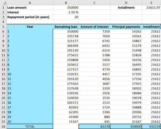

The sum of the installments should be equal to the loan amount, and you can see that this is the case here (with a small rounding error). The sum of the amount of interest you have paid is $, and the sum of all the principal payments is the sum of what you have paid back to the bank, which is $. In other words, an fixed-rate mortgage loan of $ cost you $ after 20 years.